From-scratch guide / Chapter 3 / Introductory
Gradient Descent from Scratch in Python
Gradient descent minimizes a differentiable objective by repeatedly moving the parameters opposite the gradient. In the example below, you will implement that update directly in NumPy and keep the full optimization path so you can inspect convergence.
How it works
w_(k+1) = w_k - alpha * grad g(w_k)Here w_k is the current parameter, grad g(w_k) is the local slope of the objective, and alpha is the positive step size. The minus sign makes the update move downhill.
- 1Choose an initial parameter value and a positive step size.
- 2Evaluate the gradient at the current parameter.
- 3Subtract the step-size-scaled gradient.
- 4Repeat until the gradient or parameter change is sufficiently small.
Visual intuition
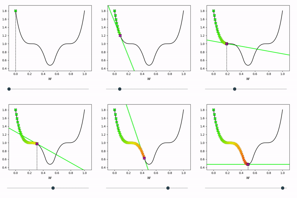
NumPy implementation
This example is deterministic and uses NumPy for arrays and arithmetic, not a prebuilt optimizer or model implementation.
import numpy as np

def objective(w):
    return (w - 3.0) ** 2

def gradient(w):
    return 2.0 * (w - 3.0)

def gradient_descent(initial_w, step_size=0.2, iterations=30):
    w = float(initial_w)
    history = [w]

    for _ in range(iterations):
        w = w - step_size * gradient(w)
        history.append(w)

    return w, np.asarray(history)

minimum, path = gradient_descent(initial_w=8.0)
The objective has its minimum at w = 3, so the example has a result we can verify exactly.
The gradient function returns the local slope; the loop contains the complete learning rule rather than calling an optimizer.
Keeping history makes the optimization path available for plotting or convergence checks.
What can go wrong
A large step can overshoot
If alpha is too large, successive updates can bounce across the minimum or diverge.
A tiny step can stall progress
A very small alpha may be stable but require far more iterations than the same objective needs with a better-scaled step.
Geometry still matters
Flat, poorly conditioned, or non-convex objectives can make first-order progress slow or lead to different stationary points.
Continue with the book and source
This guide is grounded in Chapter 3, First-Order Optimization Techniques, and the official Machine Learning Refined notebooks. Use the chapter for context, then open the exact sources below for the full treatment and exercises.