From-scratch guide / Chapter 6 / Introductory
Logistic Regression from Scratch in Python
Binary logistic regression turns a linear score into a probability with the sigmoid function, then learns the weights by minimizing binary cross-entropy. The implementation below exposes the probability, loss gradient, and thresholded prediction instead of calling a model library.
How it works
p(y=1 | x) = 1 / (1 + exp(-w^T x)); L = -mean[y log(p) + (1-y) log(1-p)]The linear score w^T x becomes a probability p through the sigmoid. Cross-entropy penalizes confident wrong probabilities, and its gradient supplies the weight update.
- 1Add a constant feature if the model needs an intercept.
- 2Compute linear scores and map them through a numerically stable sigmoid.
- 3Use the mean cross-entropy gradient X^T(p - y) / n.
- 4Update the weights, then choose a probability threshold for predictions.
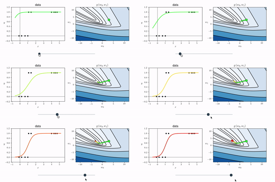
Visual intuition
NumPy implementation
This example is deterministic and uses NumPy for arrays and arithmetic, not a prebuilt optimizer or model implementation.
import numpy as np

def sigmoid(scores):
    scores = np.clip(scores, -500.0, 500.0)
    return 1.0 / (1.0 + np.exp(-scores))

def fit_logistic_regression(X, y, step_size=0.2, iterations=2000):
    X = np.asarray(X, dtype=float)
    y = np.asarray(y, dtype=float)
    weights = np.zeros(X.shape[1])

    for _ in range(iterations):
        probabilities = sigmoid(X @ weights)
        gradient = X.T @ (probabilities - y) / len(y)
        weights = weights - step_size * gradient

    return weights

def predict_proba(X, weights):
    return sigmoid(np.asarray(X, dtype=float) @ weights)

X = np.array([
    [1.0, -2.0], [1.0, -1.0], [1.0, -0.5],
    [1.0,  0.5], [1.0,  1.0], [1.0,  2.0],
])
y = np.array([0, 0, 0, 1, 1, 1])
weights = fit_logistic_regression(X, y)
predictions = (predict_proba(X, weights) >= 0.5).astype(int)
The first column of X is the intercept feature; the second contains the one-dimensional measurements.
Clipping scores keeps exp from overflowing while leaving ordinary score values unchanged.
The training loop is the full vectorized gradient method, and the threshold is applied only after probabilities are computed.
What can go wrong
Scale affects optimization
Features on very different scales can make one global step size inefficient or unstable.
The threshold is a decision choice
Changing 0.5 changes predicted labels; it does not retrain the probability model or fix class imbalance.
Probability code needs numerical care
Extreme scores can overflow exp, and direct log-loss calculations must clip probabilities or use a stable equivalent.
Continue with the book and source
This guide is grounded in Chapter 6, Two-Class Classification, and the official Machine Learning Refined notebooks. Use the chapter for context, then open the exact sources below for the full treatment and exercises.